1. Serial Numbers

If you work with large data then it’s better to add a serial number column to it. For me, the best way to do this is to apply the table (Control + 5) to the data and then add 1 in the above serial number, just like below.

To do this, you simply need to add 1 to the first cell of the column and then create a formula to add 1 to the above cell’s value.

2. Current Date and Time

The best way to insert the current date and time is to use the NOW function which takes date and time from the system and returns it.


The only problem with this function is it’s volatile, and whenever you recalculate something it updates its value. And if you don’t want to do this, the best way is to convert it to hard value.

3. Select Non-Adjacent Cell

Normally we all do it this way, hold the control key, and select cells one by one.
But I have found that there is a far better way for this. All you have do is, select the first cell and then press SHIFT + F8.


This gives you add or remove selection mode in which you can select cells just by selecting them.

4. Sort Buttons

If you deal with the data which needs to sort frequently then it’s better to add a button to the quick access toolbar (if it’s not there already).


All you need to do is click on the down arrow on the quick access toolbar and then select “Sort Ascending” and “Sort Descending”. It adds both buttons to the QAT.

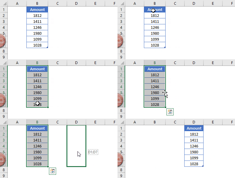
5. Drag and Drop

How to move data from one section of your worksheet to another? I’m sure you think about copy-paste but you can also use drag-drop for this.


Simply select the range where you have data and then click on the border of the selection. By holding it move to the place where you need to put it.

6. Status Bar

The status bar is always there but we hardly use it to the full. If you right-click on it, you can see there are a lot of options you can add.

7. Paste from Clipboard

When you copy a value, it goes to the clipboard and if you open the clipboard you can paste all the values which you have copied.
To open a clipboard, click on the go to Home Tab ➜ Editing and then click on the down arrow.


It will open the clipboard on the left side, and you can paste values from there.

8. Add Bullet Points

Press Ctrl + 1 and you will get the “Format Cell” dialogue box.
Under the number tab, select custom.
In the input bar, enter the following formatting.
● General;● General;● General;● General


Click OK.
Now, whenever you enter a value in the cell Excel will add a bullet before that.

9. Copy of Worksheet

To create a copy of a worksheet in the same workbook drag and drop in the best way.

10. Undo-Redo Buttons

Just like sort buttons you can also add undo and redo buttons to the QAT. The best part about those buttons is you can use them to undo up to a particular activity without pressing the shortcut key again and again.

11. Auto Format

If you deal with financial data, then auto format can be one of your best tools. It simply applies the format to small as well as large data sets (especially when data is in tabular form).

• First of all, you need to add it to the quick access toolbar.
• After that, whenever you need to apply the format, just select the data where you want to apply it and click on the AUTO FORMAT button from quick access toolbar.
• It will show you a window to select the formatting type and after selecting that click OK.

12. Format Painter

The simple idea with the format painter is to copy and paste formatting from one section to another.
Let’s say you have specific formatting (Font, Cell Color, Bold, Border, etc.) in the range B2:D7, and with format painter, you can copy that formatting to range B9: D14 with a click.

• First of all, select the range B2:D7.
• After that, go to the Home Tab ➜ Clipboard and then click on “Format Painter”.
• Now, select the cell C1 and it will automatically apply the formatting on B9: D14.

The format painter is fast and makes it easy to apply to format from one section to another. Even you can also apply formatting multiple times.

13. Cell Message

Let’s say you need to add a specific message to a cell, like “Don’t delete the value”, “enter your name” or something like that. In this case, you can add a cell message for that particular cell. When the user will select that cell, it will show the message you have specified.

Here are the steps to do this:

• First, select the cell for which you want to add a message.
• After that, go to the Data Tab ➜ Data Tools ➜ Data Validation ➜ Data Validation.
• In the data validation window, go to the Input Message tab.
• Enter title, message and make sure to tick mark “Show input message when the cell is selected”.
  
  
• In the end, click OK.
  
  

Once the message is showed you can drag and drop it to change its position.

14. Strikethrough

Unlike Word, in Excel, there is no option on the ribbon to apply strikethrough. But I have figured out that there are 5 ways to do it and easiest from all of them is a keyboard shortcut. All you need to do it select the cell where you want to apply the strikethrough and use the below keyboard shortcut.
Control + 5

15. Barcode

To create a bar-code in Excel all you need to do it install this bar-code font from ID-AUTOMATIC.


Once you install this font, you will have to type the number in a cell for which you want to create a bar-code and then apply the font style

16. Month Name

Let’s say you have a date in a cell, and you want that date to show as a month or a year. For this, you can apply custom formatting.

• First, select the cell with a date and open formatting options (use Ctrl + 1).
• Select the “Custom” option and add “MMM” or “MMMMMM” for the month or “YYYY” for the year format.
  
  
• In the end, click OK.

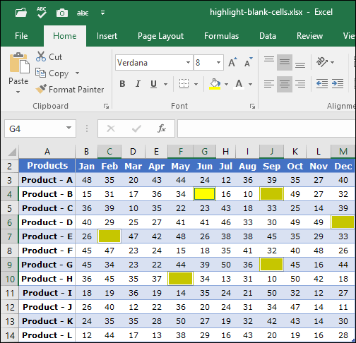
17. Highlight Blank Cells

When you work with large data sheets it’s hard to identify the blank cells from it. So, the best way is to highlight them by applying a cell color.

• First, select all the data from the worksheet using the shortcut key Ctrl + A.
  
  
• After that, go to Home Tab ➜ Editing ➜ Find & Select ➜ Go to Special.
  
  
• From Go to Special dialog box, select Blank and click OK.
  
  
• At this point, you have all the blank cell selected and now apply a cell color using font settings.
  
  

but you can also use conditional formatting for this.

18. Font Color with Custom Formatting

In Excel, we can apply custom formatting and in custom formatting, there is an option to use font colours (limited but useful). For example, if you want to use the Green colour for positive numbers and red colour for negative numbers then you need to use the custom format.
[Green]#,###;[Red]-#,###;0;

To apply this all you need to do is:

• First, select the cells where you want to apply this format.
• After that open format option using keyboard shortcut Ctrl + 1 and go to the “Custom” category and the custom format in the input dialogue box.
  
  
• In the end, click OK.

19. Theme Color

We all have some favourite fonts and colours which we use in Excel. Let’s say you received a file from your colleague and now you want to change the font and colours for the worksheet from that file. The point is, you need to do this one by one for each worksheet and that takes time.

But if you create a custom theme with your favourite colours and fonts then you can change the style of the worksheet with a single click. For this, all you have to do is apply your favourite designs to the tables, colours to the shapes and charts, font style and then save it as a custom theme.


And now, every time you need just one click to change any worksheet style to your custom style.

20. Clear Formatting

This is a simple keyboard shortcut that you can use to clear formatting from a cell or range of cells.
Alt ➜ H ➜ E ➜ F
Or, otherwise, you can also use clear formatting option from the Home Tab (Home Tab ➜ Editing ➜ Clear ➜ Formats).

21. Sentence Case

In Excel, we have three different functions (LOWER, UPPER, and PROPER) to convert a text into different cases. But there is no option to convert a text into sentences case. Here is the formula which you can use:
=UPPER(LEFT(A1,1))&LOWER(RIGHT(A1,LEN(A1)-1))


This formula converts the first letter of a sentence into capital and rest of all in small…

22. Random Numbers

In Excel, there are two specific functions which you can use to generate random numbers. First is RAND which generates random numbers between 0 and 1.


And second is RANDBETWEEN which generates the random numbers within the range of two specific numbers.


ALERT: These both functions are volatile so whenever you re-calculate your worksheet or hit enter, they update their values so make sure to use them with caution.

23. Count Words

In Excel, there is no specific function to count words.
You can count characters with LEN but not words. But, you can use the following formula which can help you to count words from a cell.
=LEN(A1)-LEN(SUBSTITUTE(A1,” “,””))+1



This formula counts the number of spaces from a cell and adds 1 to it after that which equals the total number of words in a cell.

24. Calculate Age

he best way to calculate a person’s age is by using the DATEDIF function. This mysterious function is specifically made to get the difference between two dates.



And the formula will be:
=”Your age is “& DATEDIF(Date-of-Birth,Today(),”y”) &” Year(s), “& DATEDIF(Date-of-Birth,TODAY(),”ym”)& ” MONTH(s) & “& DATEDIF(Date-of-Birth,TODAY(),”md”)& ” Day(s).”

25. Ratio

I have figured out that there are 4 different ways to calculate ratio in Excel but using a simple divide method is the easiest one. All you need to do is divide the larger number into the smaller one concatenate it with a colon and one and here’s the formula you need to use:
=Larger-Number/Smaller-Number&”:”&”1″



This formula divides the larger number with the smaller so that you can take the smaller number as a base (1).

26. Root of Number

To calculate square root, cube root or any root of a number the best way is to use exponent formula. In exponent formula, you can specify the Nth number for which you want to calculate the root.
=number^(1/n)

For example, if you want to calculate a square root of 625 then the formula will be:
=625^(1/2).

27. Days in Month

To get a total number of days in a month dynamically you can use the following formula:
=DAY(EOMONTH(TODAY(),0))

28. Month’s last Date

To simply get the last date of a month you can use the following dynamic formula.
=DATE(YEAR(TODAY()),MONTH(TODAY())+1,0)

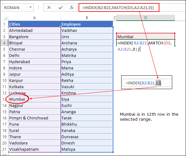
29. INDEX and MATCH

• MATCH tells the INDEX the position (cell number) of the value in a column or in a row.
• And, then the INDEX returns the value using that position (cell number).

Just think like this, MATCH function is an undercover agent who finds the criminal and INDEX function is a cop who arrests that criminal afterward. Below we have a list of cities and name of the employees who are working there. Here we need to lookup for the employee name who’s working in Mumbai.

Now, if look at data, in the column where you have cities, that is our lookup column and the column where you have employees name, that is your value column. And, the formula will be:
=INDEX(B2:B11,MATCH(E3,A2:A11,0),0)

Part-1: In the part one, we have used the match function to lookup for the value “Mumbai” and it has returned the “5” which is the position of the cell in which you have value “Mumbai” in cities column.


Part-2: In the part two, we have used INDEX and referred employees name column for lookup of the value. Here index function knows that you want value from the 12th cell from the column. So, it has return “Siya” in the result.

30. SUMPRODUCT IF

You can use the below formula to create a conditional SUMPRODUCT and product values using a condition.
=SUMPRODUCT(–(C7:C19=C2),E7:E19,F7:F19)

31. Smooth Line

If you love to use a line chart, then you are awesome but it would be more awesome if you use a smooth line in the chart. This will give a smart look to your chart.

Here are the steps:

• Select the data line in your chart and right click on it.
• Select “Format Data Series”.
• Go to Fill & Line ➜ Line ➜ Tick mark “Smoothed Line”.

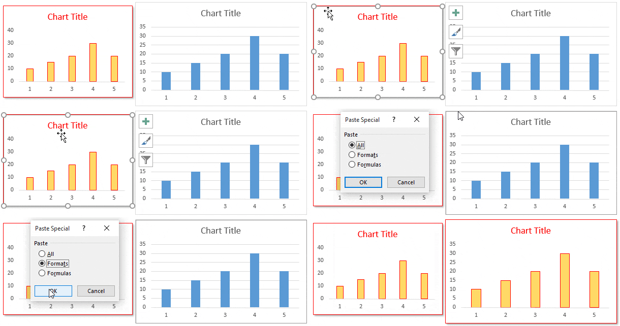
32. Chart Formatting

Steps to Copy Formatting from One Chart to Another:

1. First of all, right-click on the chart from which you want to copy the chart formatting.
2. And, then click on the copy.
3. After that, right-click on the other chart on which you want to apply/paste the formatting.
4. Now, go to Home tab -> Clipboard -> Paste -> Paste Special.
5. Here you have a pop-up window.
6. Select formats and click OK.

33. Hide Axis Labels

This charting tip is simple but still quite useful. If you don’t want to show axis label values in your chart you can delete them. But the better way is to hide them instead of deleting. Here are the steps:

• Select Horizontal/Vertical axis in the chart.
• Go to “Format Axis” Labels.
• In label position, select “None”.

And again, if you want to show it then just select “Next to axis”.

34. Display Units

If you are dealing with the large numbers in your chart, you can change the units for axis values.
Select chart axis your chart and open format “Format Axis” options.


In axis options, go to “Display Units” where you can select unit for your axis values.

35. Round Corner

I often use Excel charts with rounded corners and if you like to use round corners too, here are the simple steps.

1. Select your chart and open formatting options.
2. Go to Fill and Line ➜ Borders.
3. In borders sections, tick mark rounded corners.

36. Hide Gap

Let’s say if you have a chart with monthly sales in which Jun has no amount and cell is empty. You can use the following options for that empty cell.

• Show the gap for the empty cell.
• Use zero.
• Connect data points with the line.

Here are the steps to use these options.

• Right, click on your chart & select “Select Data”.
• In select data window, click on “Hidden and Empty Cell”.
• Select your desired option from “Show Empty Cell as”.

Make sure to use “Connect data points with the line” (recommended).

37. Pictograph in Excel

If you know how to present data in an understandable and effective way, you can deliver your message strongly. It is the total employees in a company age wise and we need to present these groups using this chart.


But before we start, we need an icon to use in this chart and you can download it from a free icon site.

1. First of all, just select your data to create a bar chart. For this, go to Insert ➜ Charts ➜ 2-D Clustered Bar Chart.
   
   
2. After that, select the data bars in the chart and go to Right Click ➜ Format Data Series Option
   
   
3. From here, go to “Fill” section and select “Picture or Texture Fill” option and once you do this, you’ll get an insert picture option.
   
   
4. Now it’s time to insert the picture and we have three options for this. Click on the “File” option and upload the image you have downloaded.
5. Once you insert the image, you have further three options to show that picture in the chart. [Select the third option]
   i) Stretch – A single image will stretch in data bar.
   ii) Stack – You will get stacked images in the data bar.
   iii) Stack and Scale with – Images will be shown as per data.

Now our chart is ready to rock.

Note: There is an option to specify unit/picture for the chart. You can use it if the values per bar in your chart are large (more than 20). The thing is that the picture icons will become smaller with more numbers and this option helps in that case.


You can also use a different picture for different bars. Select each data bar separately and insert a picture one by one for all the bars.

38. Chart Template

Let’s say if you have a favourite chart formatting which you want to apply every time you create a new chart. You can create a chart template to use it anytime in the future and steps are as follow.

1. Once you have done with your favourite formatting, right click on it & select “Save As Template”.
   
   
2. Using save as dialog box, save it in the template folder.
3. To insert a new with your favourite template, select it from templates in insert chart dialog.
   
   

39. Default Chart

You can use a shortcut key to insert a chart, but the problem is, it will only insert the default chart, and in Excel, the default chart type is “Column Chart”. So if your favourite chart is a line chart, then the shortcut is useless for you. But let’s conquer this problem. Here are the steps to fix this:

1. Go to Insert Tab ➜ Charts.
2. Click on the arrow at the bottom right corner.
3. Then in your insert chart window, go to “All Charts” and then select the chart category.
4. Right, click on the chart style which you want to make your default Select “Set as Default Chart”. Then click OK.

40. Hidden Cells

When you hide a cell from the data range of a chart, it will also hide that data point from the chart as well. To fix this, just follow these steps.

1. Select your chart and right click on it.
2. Go to ➜ Select Data ➜ Hidden and empty cells.
3. From the pop-up window, tick mark “Show data in hidden rows and columns”.
   
   

41. Print Titles

Let’s say you have headings in your table, and you want to print those headings on every page you print. In this case, you can fix “Print Titles” to print those headings on each page.

• Go to “Page Layout Tab” ➜ Page Set Up ➜ Click on Print Titles.
• Now in the page setup window go to sheet tab and specify following things.
  
  

1. Print Area: Select the entire data which you want to print.
2. Rows to repeat at the top: Heading row(s) which you want to repeat on every page.
3. Columns to repeat at the left: Column(s) which you want to repeat at the left side of every page (if any).
   
   

42. Page Order

Specifying the page order is quite useful when you want to print large data.

• Go to File Tab ➜ Print ➜ Print Setup ➜ Sheets Tab.
• Now here, you have two options:
  i) The First Option: To print your pages using a vertical order.
  ii) The Second Option: To print your pages using a horizontal order.
  
  

43. Print Comments

If you use comments in your reports then you can print them as well. At the end of all printed pages, you can get a list of all the comments.

• Go to File Tab ➜ Print ➜ Print Setup ➜ Sheets Tab.
• In the print section, select “At the end of the sheet” using comment dropdown.
• Click OK.

44. Scale to Fit

Sometimes we struggle to print entire data on a single page. In this situation, you can use the “Scale to Fit” option to adjust the entire data into a single page.

1. Go to File Tab ➜ Print ➜ Print Setup ➜ Page Tab.
2. Next, you need to adjust two options:
   i) Adjust % of normal size.
   ii) Specify the number of pages in which you want to adjust your entire data using width and length.
   
   

45. Custom Header-Footer

Instead of using the page number in the header and footer, you can also use a custom header and footer.

• Go to File Tab ➜ Print ➜ Print Setup ➜ Header/Footer.
• Click on custom header or footer button.
  
• Here you can select alignment of the header/footer.
  
  
• And the following options can be used:
  1. Page Number
  2. Page Number with total pages.
  3. Date
  4. Time
  5. File Path
  6. File Name
  7. Sheet Name
  8. Image

46. Center on Page

Imagine you have fewer data to print on a page. In this case, you can align it at the center of the page while printing.

• Go to File Tab ➜ Print ➜ Print Setup ➜ Margins.
• In “Center on Page” you have two options to select.
  I) Horizontally: Aligns data to the center of the page.
  ii) Vertically: Aligns data to the middle of the page.
  
  

47. Print Area

The simple way to print a range is to select that range and use the option “print selection”.
But what if you need to print that range frequently, in that case you can specify the printing area and print it without selecting it every time.

48. Custom Margin

• Go to File Tab ➜ Print.
• Once you click on print, you’ll get an instant print preview.
• Now from the bottom right side of the window, click on “Show Margins” button.
  
  

It will show all the margins applied and you can change them just by drag and drop.

49. Error Values

You can replace all the error values while printing with a specific value (three other values to use as a replacement). Here are the steps:

• Go to File Tab ➜ Print ➜ Print Setup ➜ Sheet.
• Select replacement value from “Cell error as” drop down.
• You have three options to use as a replacement.
  1. Blank
  2. Double minus sign.
  3. “#N/A” error for all the errors.
  
  
• After selecting the replacement value, click OK.

I think using “Double minus sign” is the best way to present errors in a report while printing it on a page.

50. Custom Start Page Number

If you want to start page number from a custom number let’s say 5. You can specify that number and rest of the pages will follow that sequence.

• Go to File Tab ➜ Print ➜ Print Setup ➜ Page.
• In the input box “First page Number”, enter the number from where you want to start the page number.
  
  
• In the end, click OK.
• After selecting the replacement value, click OK.

Important Note: This option will only work if you have applied header/footer in your worksheet.

51. Tracking Important Cells

Sometimes we need to track some important cells in a workbook and for this, the best way is to use the watch window. In the watch window, you add those important cells and then get some specific information about them in one place (without navigating to each cell). Here are the steps to use it:

• First, go to Formula Tab ➜ Formula Auditing ➜ Watch Window.
  
  
• Now in “Watch Window” dialog box, click on “Add Watch”.
  
  
• After that select the cell or range of cells that you want to add and click OK.

Once you hit OK, you’ll some specific information about the cell(s) in the watch window.

52. Flash Fill

It’s like a copycat, perform the task which you have performed. Let me give you an example.


Here are the steps to use it:
You have dates in the range A1: A10 and now, you want to get the month from the dates in the B column.
All you need to do is to type the month of the first date in the cell B1 and then come down to cell B2 and press the shortcut key CTRL + E.

Once you do this it will extract the month from the rest of the dates, just like below.

53. Combine Worksheets

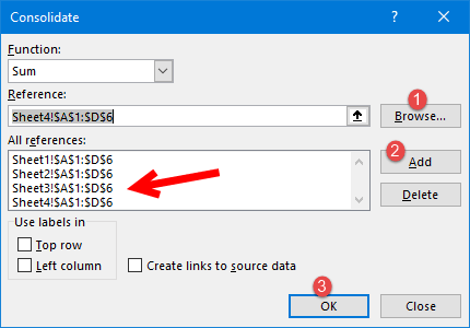
I’m sure somewhere in the past you have received a file from your colleague where you have 12 different worksheets for 12 months data. In this case, the best solution is to combine all of those worksheets using the “Consolidate” option and here are the steps for this.

• First, add a new worksheet and then go to Data Tab ➜ Data Tools ➜ Consolidate.
  
  
• Now in the “Consolidate” window, click on the upper arrow to add the range from the first worksheet and then click on the “Add” button.
• Next, you need to add references from all the worksheets using the above step.
  
  
• In the end, click OK.

54. Live Image

In Excel, using a live image of a table can help you resize it according to space and to create a live image there are two different ways which you can use. One is camera tools and the second is the paste special option. Here the steps to use camera tool and for paste special use the below steps.

• Select the rage you want to paste as an image and copy it.
• Go to the cell and right click, where you want to paste it.
• Go to Paste Special ➜ Other Paste ➜ Options Linked Picture.
  
  

Make sure to read this guide about camera tool to learn more about linked images.

55. Protect a Workbook

Adding a password to a workbook is quite simple, here are the steps.

• While saving a file when you open a “Save As” dialog box go to Tools General Options.
  
  
• Add a password to for “Password to Open” and click OK.
  
  
• Re-enter the password and click OK again.
• In the end, save the file.

Now, whenever you re-open this file it will ask you to enter the password to open it.

56. Userform

A few of the Excel users know that there is a default data entry form is there which we can use. And the best part is there is no need to write a single line of code for this.

• First of all, make sure you have a table with headings where you want to enter the data.
• After that select any of the cell from that table and use the shortcut key Alt + D + O + O to open the user form.

57. Custom Tab

We all some favorite option or some options which we use frequently. To access all those options in one place you create tab and add them to it. Follow these steps:

• First, go to File Tab ➜ Options ➜ Customize Ribbon.
  
  
• Now click on “New Tab” (this will add a new tab).
• After that right click on it and name it and then name the group.
• Finally, we need to add options to the tab and for this go to “Choose Commands From” and add them to the tab one by one.
• In the end, click OK.

Now you are a new tab in the Excel ribbon with all the favorite options.

58. Goal Seek

In simple words, Goal Seek is a problem-solving tool. It helps you find the input value by proving the value you want in the result.

59. Text to Speech

This is an option where you can make Excel speak the text you have entered into a cell or a range of cells.

60. Named Range

To create a named the range the easiest method is to select the range create it using the “Create from Selection” option. Here are the steps to do this:

• Select the column/row for which you want to create a named range.
• Right click and click on “Define name…”.
  
  
• Select the option to add the name for the named range and click OK.
  
  

61. Trim

TRIM can help you to remove extra spaces from a text string. Just refer to the cell from where you want to remove the spaces and it will return the trimmed value in the result.

62. Remove Duplicates

One of the most common things which we face while working with large data is “Duplicate Values”. In Excel, to remove these duplicate values is quite simple. Here’s how to do this.

• First, select any of the cells from the data or select the entire data.
  
  
• After that, go to Data ➜ Data Tools ➜ Remove Duplicates.
• At this point, you have “Remove Duplicates” window and from this window, select/de-select the columns which you want to consider/not consider while removing duplicate values.
• In the end, click OK.

Once you click OK, Excel will remove all the rows from the selected data where values are duplicate and show a message with the number of values removed and unique values left.

63. Combine Text (Fill Justify)

I know five different ways to merge text from a range but out of those Fill Justify is my favorite. It’s one of the less used options in Excel, but worth not to be missed for any reason. Let say you have words in the range A1: A5 and you want to concatenate all of them in a single cell. Here’s how to do this with fill justify.

• First, make column A enough wide so that the entire text can be combined into one cell.
• After that, select the entire range.
• Now, go to Home Tab ➜ Editing ➜ Fill ➜ Justify.

It combined the text from range A1:A5 to cell A1.

64. Remove Specific Character

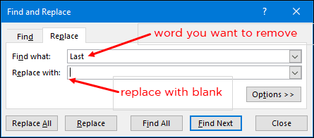
Let’s say you have some text values in a column and from those values you want to replace a specific character or a word… You can do this simply by find and replace option. Let say you have words in the range A1: A5 and you want to concatenate all of them in a single cell. Here’s how to do this with fill justify.

• All you need to do is select that column and open the find and replace dialog box.
• After that click on the “Replace” tab.
  
  
• Now here, in “Find What” enter the character you want to replace and make sure to leave “Replace with” blank.
• Now click on “Replace All”.

The moment you click on “Replace All” Excel will remove that particular character from the entire column.

65. Combine Text

So, you have text in multiple cells, and you want to combine all the text into one cell. No, this time not with fill justify. We are doing it with TEXT JOIN. If you use Office 365, there is new function TEXTJOIN which is a game changer when it comes to the concatenation of text.

TEXTJOIN(delimiter, ignore_empty, text1, [text2], …)

All you need to do is to add a delimiter (if any), and TRUE if you want to ignore empty cells, and in the end, refer to the range.

66. Unpivot Data

Look at the below table you can use it as a report but can use you use it further as a raw data. No, you can’t. But if you convert this table in something like below you can use it easily anywhere.


And to unpivot data, the best way is to use the POWER QUERY.

67. Delete Error Cells

Mostly while working with large data it obvious to have error values but it’s not good to keep them. The easiest way to deal with these error values is select them and delete them and these are the simple steps.

• First of all, go to Home Tab ➜ Editing ➜ Find & Replace ➜ Go To Special.
• In the Go To dialog box, select formula, and tick mark errors.
  
  
• In the end, click OK.

Once you click OK it will select all the errors and then you can simply delete all by using “Delete” button.

68. Arrange Columns

Let’s say you want to arrange columns from the data using a custom order. The normal way is to cut and paste them one by one. But we also have an out of the box way.
In Excel, you can sort columns just like you sort rows and by using the same methods you can arrange them in a custom order.

69. Convert to Date

Sometimes you have dates which are stored as text and you can use them in a calculation and further analysis. To simply convert them back to valid dates you can use DATEVALUE function…

70. Negative to Positive

71. Format Painter

Before I started to use format painter for applying cell formatting, I was using paste special with the shortcut key. Here’s how to do this:

1. Select the cell or a range from where you want to copy cell formatting.
2. Go to ➜ the Home Tab ➜ Clipboard.
3. Now, make a double click on the “Format Painter” button.
4. As soon as you do this, your cursor will convert into a paintbrush.
5. Now, you can apply that formatting anywhere in your worksheet, in another worksheet or, even in another workbook.

72. Rename a Worksheet

I always found it quicker than using a shortcut key to change the name of a worksheet. All you have to do is just double click on the sheet tab and enter a new name.


Before you change the name of a worksheet, you need to activate it. But if you use the mouse it will automatically activate that worksheet and edit the name with only two clicks.

73. Fill Handle

I am sure shortcut addicts always use a shortcut key to drag formulas and values in downward cells. But using a fill handle is more impressive than using a shortcut key.

• Select the cell in which you have a formula or a value which you want to drag.
• Make a double click on the small square box at the right bottom of the cell selection border.

This method only works if you have values in corresponding column and it works only in the vertical direction.

74. Hide Ribbon

If you want to work in a distraction-free mode, you can do this by collapsing your Excel ribbon.


Just make a double click on the active tab in your ribbon and it will collapse the ribbon. And if you want to expand it back just double click on it again.

75. Edit a Shape

You often use shapes in our worksheets to present some messages and you have to insert some text into those shapes. Besides the typical method, you can use double click to edit a shape and insert the text into it.


You can also use this method to edit and enter text in a checkbox or into a chart title.

76. Column Width

Whenever you have to adjust column width you can double click on the right edge of the column header. It auto sets the column width according to the column data.


The same method can be used to auto adjust row width.

77. Go to the Last Cell

This trick can be useful if you are working with a large dataset. By using a double click, you can go to the last cell in the range which has data.


You have to click on the right edge of the active cell to go to the right side & on the left edge if you want to go to the right side.

78. Chart Formatting

If you use Control + 1 to open formatting options to format a chart, then I bet you’ll love this trick. All you have to do is just make a double-click on the border of the graph to open formatting option.

79. Pivot Table Double Click

Let’s say someone sent you a pivot table without the source data. As you already know Excel stores data in pivot cache before creating a pivot table.


You can extract data from a pivot table by double-clicking on data values. As soon as you do this Excel will insert a new worksheet with the data which has used in the pivot table.

80. Right Click Menu

There is a right-click drop-down menu in Excel which few users know about. To use this menu all you need to do is select a cell or a range of the cell and then right-click and while holding it, drop the selection to somewhere else.

81. Default File Saving Location

Normally while working on Excel I create more than 15 Excel files every day. And, if I save each of these files to my desktop it looks nasty. To solve this problem, I have changed my default folder for saving a workbook and here’s you can do this.

1. First, go to the file tab and open Excel options.
   
   
2. In Excel options, go to “Save” category.
3. Now, there is an input bar where you can change the default local file location.
4. From this input bar, change the location address and in the end, click OK.

From now onward, when you open “Save As” dialog box Excel will show you the location you have specified.

82. Disable Start Screen

I’m sure just like me you hate when you open Microsoft Excel (or any other Office app) and you see the start pop-up screen. It takes time depending on your system’s speed and add-ins you have installed. Here are the steps to disable the start-up screen in Microsoft Office.

• First, go to the File tab and open Excel options.
• In Excel options, go to the “General” category.
• From option, drill down to “Start-Up” options and un-tick the “Show the Start screen when this application starts”.
  
  
• In the end, click OK.

From now onward, every time when you start Excel it will directly open the workbook without showing the start-up screen.

83. Developer Tab

Before you start writing VBA codes the first thing you need to do is to enable “Developer Tab”. When you first install Microsoft Excel, developer wouldn’t be there. So, you need to enable it from settings.

• First, go to File tab and click on “Customize Ribbon” category.
• Now from the tab list, tick marks the developer tab and click OK.
  
  

Now when you come back to your Excel window, you’ll have a developer tab on the ribbon.

84. Enable Macros

When you open a macro-enabled file, you need to enable macro options to run VBA codes. Follow these simple steps:

1. First, go to the File tab and click on the “Trust Center” category.
2. From here click on “Trust Center Settings”.
3. Now in “Trust Center Settings”, click on macro settings.
   
   
4. After that, click on “Enable all macros with Notifications”.
5. In the end, click OK.

85. AutoCorrect Option

With the auto correct option, you can tell Excel to change a text string into another when you type it. Follow these simple steps:

1. First, go to the File tab and go to options and click on “Proofing” category.
2. After that, click on “AutoCorrect Option” and this will open the ‘auto-correct window’.
3. Here in this window, you have two input bars to specify the text to replace and text to replace with.
   
   
4. Enter both values and then click OK.

86. Custom List

Just think like this, you have a list of 10 products which you sell. Whenever you need to insert those product name you can insert them using a custom list. Let me tell you how to do this:

1. First, go to File tab and go to options and click on “Advanced” category.
2. Now, drill down and go to “General” section and click on “Edit Custom List…”.
3. Now in this window, you can enter the list, or you can also import it from a range of cells.
   In the end, click OK.

Now, to enter the custom list you have just created, enter the first entry of the list in cell and then drill down that cell using fill handle.

87. Apply Table

If you use pivot tables a lot then it’s important to apply the table to the raw data. With a table, there is no need to update the pivot table’s data source and it drag-down formulas automatically when you add a new entry.


To apply table to the data just use Ctrl + T keyboard shortcut key and click OK.

88. Gridline Color

If you are not happy with the default color of cell grid-lines then you can simply change it with a few clicks and follow these simple steps for this:

• First, go to File tab and click on “Advanced” category.
• Now, go to “Display options for this workbook” section and select the color you want to apply.
  
  
• In the end, click OK.

89. Pin to Taskbar

This is one of my favorite one-time set up to save time in the long run. The thing is instead of going to start menu to open Microsoft Excel, the best way is to pint it to the task-bar.


This way you can open it by clicking on the icon from the taskbar.

90. Macro to QAT

If you have a macro code which you need to use frequently. Well, the easiest way to run a macro code is to add it to the quick access toolbar.

1. First, go to the File tab and click on the “Quick Access Toolbar” category.
2. After that, from “Choose Command from”, select Macros.
3. Now select the macro (you want to add to QAT) and click on add.
4. From here click on “Modify” and select an icon for the macro button.
5. In the end, click OK.

91. Select Formula Cells

Let’s say you want to convert all the formulas into values and the cells where you have formulas are non-adjacent. So instead of selecting each cell one by one, you can select all the cells where you have a formula. Here are the steps:

• First, go to Home Tab ➜ Editing ➜ Find & Select ➜ Go To Special.
• In “Go To Special” dialog box, select formulas and click OK.
  
  

92. Multiply using Paste Special

To do some one-time calculations you can use paste special option and save yourself from writing formulas.

93. Highlight Duplicate Values

Well, you can use a VBA code to highlight values but the easiest way is to use conditional formatting. Here are the steps you need to follow:

• First of all, select the range of where you want to highlight the duplicate values.
• After that, go to Home Tab ➜ Styles ➜ Highlight Cells Rule ➜ Duplicate Values.
  
  
• Now from the dialog box, select the color to use and click OK.

Once you click OK, all the values which are duplicate will get highlighted.

94. Quick Analysis

If you ever noticed that when you select a range of cell in Excel, a small icon at the bottom of the selection appears. This icon called “Quick Analysis”.


When you click on this icon you can see some of the options which are there on the ribbon which you can directly use from here to save you time.

95. RUN Command

you can also open your Excel application using RUN command.

• For this, all you have to do is open RUN (Window Key + R) and then type “excel” into it.
  
  
• In the end, hit enter.

96. Open Specific File

I’m sure like me you also have few or maybe one those kinds of workbooks which you open every day when you start working on Excel. There is an option in Excel which you can use to open a specific file(s) every time when you start Excel in your system. Here are the steps.

• Go to File ➜ Options ➜ Advanced ➜ General.
• In general, enter the location (yes, you have to type) of the folder where you have those file(s) in “At startup open all the files in”.
  
  

97. Open Excel Automatically

Whenever I “Turn ON” my laptop the first thing I do is to open Excel and I’m sure you do the same thing. Well, I’ve got a better idea here, you can add Excel to your system’s startup folder.

1. First, open “File Explorer” by using Windows key + E.
2. Now, enter the below address into the address bar to open the folder (change the username with your actual username).
   C:UsersPuneet GogiaAppDataRoamingMicrosoftWindowsStart MenuProgramsStartup
3. After that, open the Start Screen, right-click the Excel App, and click Open file location.
4. From the location (Excel App Folder), copy the Excel App icon and paste it into the “Startup” folder.

Now every time when you open your system, Excel will automatically start.

98. Smart Look Up

In Excel, there is an option called “Smart Lookup” and with this option, you can look up for text on the internet. All you have to do is, select a cell or a text from a cell, and go to Review ➜ Insights ➜ Smart Lookup.


Once you click on it, it opens a side pane where you’ll have information about that particular text which you have selected. The idea behind this option is to get information by seeing definition, images for the topic (text) from different online sources.

99. Screen Clipping

Sometimes you need to add screenshots into your spreadsheet. And for this, Excel has an option that can capture screen instantly, and then you can paste it into the worksheet. For this go to ➜ Insert ➜ Illustrations ➜ Screen Clipping.

100. Locate a Keyboard Shortcut

If you use Excel 2007 to Excel 2016, then you can locate a keyboard shortcut by pressing ALT key. Once you press it, it shows the keys for the options which are there on the ribbon, just like below.


Let say, you want to press the “Wrap Text” button, the key will be ALT H W. In the same way you can reach to all the option using the shortcut keys.