Formula and Functions
Enter a Formula | Edit a Formula | Operator Precedence | Copy/Paste a Formula | Insert Function | Top 10 Functions
A formula is an expression which calculates the value of a cell. Functions are predefined formulas and are already available in Excel.
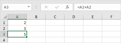
For example, cell A3 below contains a formula which adds the value of cell A2 to the value of cell A1.
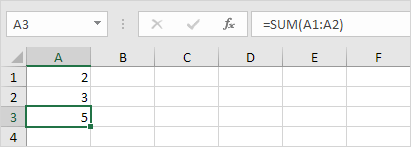
For example, cell A3 below contains the SUM function which calculates the sum of the range A1:A2.
Enter a Formula
To enter a formula, execute the following steps.
1. Select a cell.
2. To let Excel know that you want to enter a formula, type an equal sign (=).
3. For example, type the formula A1+A2.

Tip: instead of typing A1 and A2, simply select cell A1 and cell A2.
4. Change the value of cell A1 to 3.
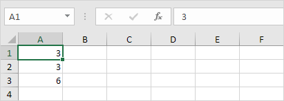
Excel automatically recalculates the value of cell A3. This is one of Excel’s most powerful features!
Edit a Formula
When you select a cell, Excel shows the value or formula of the cell in the formula bar.
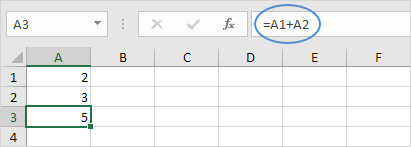
1. To edit a formula, click in the formula bar and change the formula.
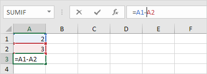
2. Press Enter.
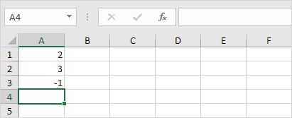
Operator Precedence
Excel uses a default order in which calculations occur. If a part of the formula is in parentheses, that part will be calculated first. It then performs multiplication or division calculations. Once this is complete, Excel will add and subtract the remainder of your formula. See the example below.
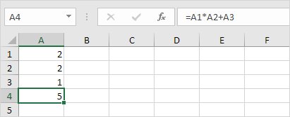
First, Excel performs multiplication (A1 * A2). Next, Excel adds the value of cell A3 to this result.
Another example,
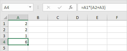
First, Excel calculates the part in parentheses (A2+A3). Next, it multiplies this result by the value of cell A1.
Copy/Paste a Formula
When you copy a formula, Excel automatically adjusts the cell references for each new cell the formula is copied to. To understand this, execute the following steps.
1. Enter the formula shown below into cell A4.
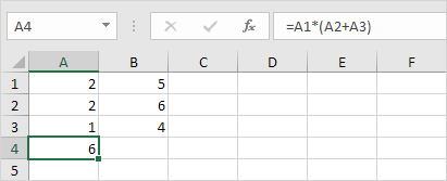
2a. Select cell A4, right click, and then click Copy (or press CTRL + c)…

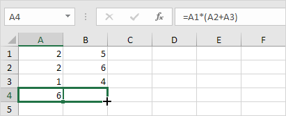
…next, select cell B4, right click, and then click Paste under ‘Paste Options:’ (or press CTRL + v).

2b. You can also drag the formula to cell B4. Select cell A4, click on the lower right corner of cell A4 and drag it across to cell B4. This is much easier and gives the exact same result!
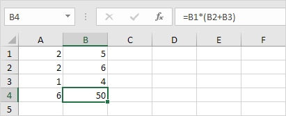
Result. The formula in cell B4 references the values in column B.
Insert Function
Every function has the same structure. For example, SUM(A1:A4). The name of this function is SUM. The part between the brackets (arguments) means we give Excel the range A1:A4 as input. This function adds the values in cells A1, A2, A3 and A4. It’s not easy to remember which function and which arguments to use for each task. Fortunately, the Insert Function feature in Excel helps you with this.
To insert a function, execute the following steps.
1. Select a cell.
2. Click the Insert Function button.

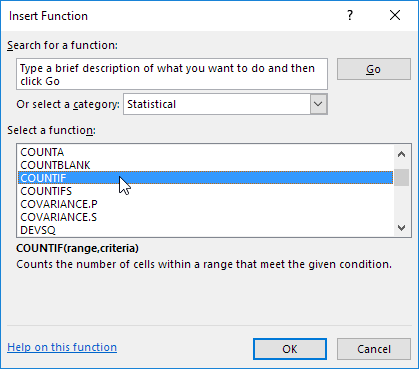
The ‘Insert Function’ dialog box appears.
3. Search for a function or select a function from a category. For example, choose COUNTIF from the Statistical category.
4. Click OK.
The ‘Function Arguments’ dialog box appears.
5. Click in the Range box and select the range A1:C2.
6. Click in the Criteria box and type >5.
7. Click OK.
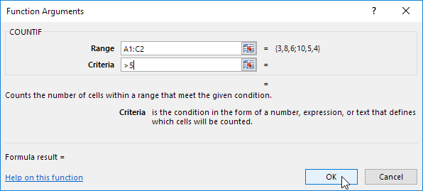
Result. The COUNTIF function counts the number of cells that are greater than 5.

Note: instead of using the Insert Function feature, simply type =COUNTIF(A1:C2,”>5″). When you arrive at: =COUNTIF( instead of typing A1:C2, simply select the range A1:C2.
Top 10 Functions
Microsoft Excel is all about formulas and functions. Below you can find an overview of the 10 most used Excel functions (+ extra tricks when creating formulas in Excel).
1. COUNT
To count the number of cells that contain numbers, use the COUNT function.

Note: use COUNTBLANK and COUNTA to count blank/nonblank cells in Excel. COUNTA stands for count all.
2. SUM
To sum a range of cells, use the SUM function (see second image on this page). You can also use the SUM function in Excel to sum an entire column.


Note: =SUM(5:5) sums all values in the 5th row. To create awesome SUM formulas, combine the SUM function with other Excel functions.
3. IF
The IF function checks whether a condition is met, and returns one value if true and another value if false.

Explanation: if the score is greater than or equal to 60, the IF function returns Pass, else it returns Fail. Remember, to quickly copy this formula to the other cells, click on the lower right corner of cell C2 and drag it down to cell C6.
4. AVERAGE
To calculate the average of a group of numbers, use the AVERAGE function (no rocket science here). The formula below calculates the average of the top 3 numbers in the range A1:A6.

Explanation: the LARGE function returns the array constant {20,15,10}. This array constant is used as an argument for the AVERAGE function, giving a result of 15.
5. COUNTIF
The COUNTIF function below counts the number of cells that contain exactly star + a series of zero or more characters.

Explanation: an asterisk (*) matches a series of zero or more characters. Visit our page about the COUNTIF function for more information and examples.
6. SUMIF
The SUMIF function below sums values in the range B1:B5 if the corresponding cells in the range A1:A5 contain exactly circle + 1 character.

Explanation: a question mark (?) matches exactly one character. Visit our page about the SUMIF function for more information and examples.
7. VLOOKUP
The VLOOKUP function below looks up the value 53 (first argument) in the leftmost column of the red table (second argument). The value 4 (third argument) tells the VLOOKUP function to return the value in the same row from the fourth column of the red table.

Note: visit our page about the VLOOKUP function to learn more about this powerful Excel function.
8. INDEX and MATCH
Use INDEX and MATCH in Excel to perform advanced lookups (if you’re new to Excel, you can skip this formula). For example, use INDEX and MATCH to perform a two-column lookup.

Note: the array formula above looks up the salary of James Clark, not James Smith, not James Anderson. Learn how to use INDEX and MATCH in Excel and impress your boss.
9. MIN and MAX
To find the minimum value, use the MIN function. To find the maximum value, use the MAX function. It’s as simple as it sounds.


Note: visit our chapter about statistical functions to learn much more about Excel and Statistics.
10. SUMPRODUCT
To calculate the sum of the products of corresponding numbers in one or more ranges, use Excel’s powerful SUMPRODUCT function.

Explanation: the SUMPRODUCT function performs this calculation: (2 * 1000) + (4 * 250) + (4 * 100) + (2 * 50) = 3500. The SUMPRODUCT function is an extremely versatile function and can produce the same result as many built-in functions in Excel and even array formulas!


